Autonomous system

Processes

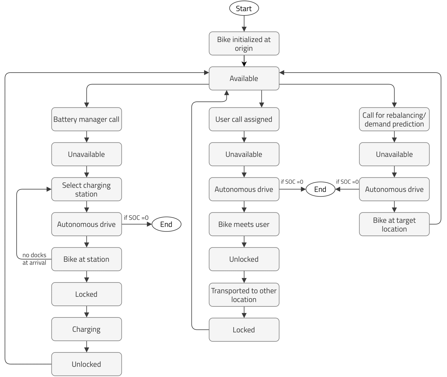
The autonomous bike process has three main sub-routines: a) user call request, b) battery management, and c) rebalancing management.

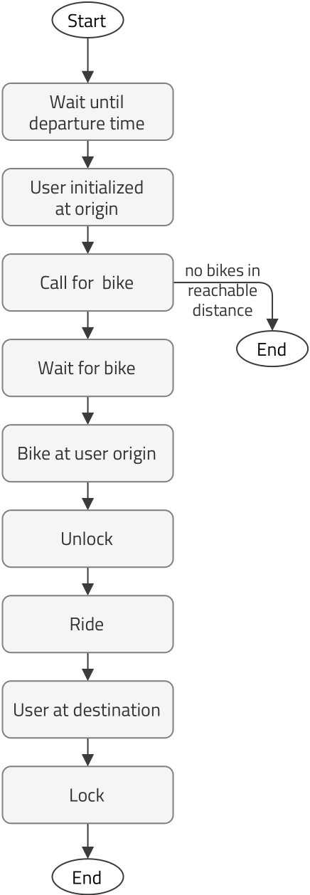
The user call sub-routine is very similar to the one in the station-based system, except that the user does not walk to the station, but rather the bike drives autonomously to the user location. With autonomous bicycles, the user requests a bicycle, and the system assigns the nearest available bicycle to this user. The user has to wait while the bicycle drives autonomously to pick them up. If the wait time is too long, the system does not assign a bicycle, and the user has to choose another mode of transportation. When the bike arrives at the user's location, they will ride it as if it was a regular bicycle before dropping it off at the destination location.

Concerning battery management, the bike is sent to a charging station whenever the battery level falls below a predefined minimum value. These charging stations are similar to station-based docking stations, with the main difference being that they are used to charge autonomous bikes. In the current simulation, charging stations are located in the exact same locations as docking stations. While it is beyond the scope of this paper, the number and location of the charging stations could be optimized based on bicycle usage. The battery level is checked right after a user locks the bike or in case the rebalancing system is activated after a bike has been rebalanced.

The third sub-routine corresponds to bike rebalancing management. In this regard, for this simulation, two extreme scenarios are implemented. One in which there is no rebalancing, and the bikes stay wherever the last user left them until they receive a call. The other scenario represents an ideal rebalancing in which there would be a perfect demand prediction model and routing algorithm. In this case, whenever a user calls for a bike, a bike immediately appears at the user's location. While this transition is supposed to be immediate, the distance traveled and the battery consumption are considered in the simulation. The real behavior is expected to be in-between scenarios; therefore, the scenario with no rebalancing and the scenario with ideal rebalancing provide, respectively, a lower- and upper- bound to the performance metrics.

It should be noted that the autonomous drive sub-routine can be commanded by the rebalancing manager, the charging manager, or a user call. The battery level is discharged in proportion to the traveled distance.

The configuration parameters for autonomous systems are:

Parameter	Description	Units
"MODE"	0=Station-based, 1=Dockless, 2= Autonomous	[-]
"NUM_BIKES"	Number of bikes in the system, fleet size	[-]
"AUTONOMOUS_RADIUS"	Maximum distance that an autonomous bike will do to pick up a user	[m]
"RIDING_SPEED"	Average bike riding speed of users	[km/h]
"AUTONOMOUS_SPEED"	Average speed of the bike in autonomous mode	[km/h]
"BATTERY_MIN_LEVEL"	Level at which the autonomous bikes go to a charging station	[%]
"BATTERY_AUTONOMY"	Autonomy of the autonomous bikes	[km]
"BATTERY_CHARGE_TIME"	Time that it takes to charge a battery from 0 to 100%	[h]

Demand prediction module

In a fleet of autonomous bicycles, reaching a perfect system efficiency and service quality would require instantly arranging a bike at the location demanded by each user. This level of performance is not possible to achieve with limited cost and fleet sizes. However, bikes can move around the city by taking advantage of their autonomous technology, locating themselves closer to high-demand areas, and, consequently, balancing the system. In that way, users would receive better average service and faster access to autonomous bikes. There are two requirements for providing an autonomous BSS fleet with such rebalancing capabilities: a demand prediction module and a routing optimization algorithm. In this section, the approach followed for the task of demand prediction is described.

The demand prediction module informs the rebalancing manager where users' demand will occur in the near future.The demand function $f$ is a mapping from the continuous 2D plane space to a scalar in the natural numbers: $f: \mathbb{R}^2 \rightarrow \mathbb{N}$. To facilitate the demand prediction, first the urban 2D space is discretized into a finite number of cells. Cells can be of any shape and size. For this implementation, Uber's hexagonal hierarchical spatial index (H3) [1] with resolution level 8 was selected, yielding 180 hexagonal cells.

A demand prediction model for each cell separately fails to utilize hidden correlations between cells to enhance prediction performance. Therefore, for the task of demand prediction, a Graph Convolutional Neural Networks with Data-driven Graph Filter (GCNN-DDGF) [2] was applied. The main limitation of a GCNN [3] is that its performance relies on a pre-defined graph structure. The GCNN-DDGF model, on the contrary, can learn hidden heterogeneous pairwise correlations between grid cells to predict cell-level hourly demand in a large-scale bike-sharing network. The GCNN-DDGF model is enhanced with a Negative Binomial probabilistic neuron at the last layer of the neural topology.

The simulation experiments were applied to the city of Boston. The bike-sharing demand dataset includes over 4.2 million bike-sharing transactions between 01/01/2018 and 31/12/2019, which are downloaded from Bluebikes Metro Boston's public bike share program. The dataset was split at date 31/09/2019 into the train (01/01/2018-31/09/2019) and test (01/10/2019-21/12/2019) sets and was processed as follows: for each cell, 70080 (2 years x 365 days x 24 hours x 4) 15-minute bike demands were aggregated based on the bike check-out time and start station in transaction records. After preprocessing, as 180 hexagonal cells were considered in this study, a 180 by 70080 matrix was obtained. The input to the model is a window of $W$ data points (each point representing 15 minutes), and the output is computed $P$ data points ahead of time. Finally, the prediction model is invoked every $T$ data points. These three parameters, input window $W$, prediction ahead $P$, and prediction period $T$, were implemented on the simulation so that the rebalancing manager can customize this service. The model performance was evaluated using the Root Mean Square Error (RMSE) as the main criteria. The testing RMSE for the trained GCNN-DDGF model on Boston data was $2.69$.

This performance metric is very close to the results obtained by the original implementation by Lin et al. [2], with a testing RMSE of $2.12$. The model training task was conducted using Tensorflow, an open-source deep learning neural network library, with Python 3.7.4 in a Ubuntu 18.04 Linux system with 64 GB RAM and GTX 1080 graphics card.

The procedure that was followed to generate the demand prediction file is the following:

1. Download the historical trip data from Bluebikes and save it in a folder ‘bluebikes_data’ within the Preprocessing folder

2. Rscript training_data.R (input bluebikes_data → outputs training_data.csv)

3. python3 gccn_ddgf.py (input training_data.csv → outputs testing_data.csv)

4. Rscript testing_data.R (input testing_data.csv → outputs demand_grid.csv)

Bike Rebalancing Transportation Problem

The demand prediction module alone is not enough to generate an efficient rebalancing algorithm. A routing optimization algorithm is necessary to minimize the global transport costs between a set of supply points and a set of demand points. %In this section, the selected routing optimization algorithm is presented. $T_{i,j}\geqslant0$ represents the number of bikes transported from supply point $i$ (with $B_{i}\geqslant0$ bikes available) to demand point $j$ (that requires $D_{j}\geqslant0$ bikes). Taking into account the number of bikes in each cell $B_{i}$, a unbalanced Hitchcock–Koopmans transportation problem is solved to yield the optimal flow of bikes between each pair of cells.

Review

Do we have the hex cells in the code? Review Figure XX below: the figure below just represent the transition matrix between two cells. It does not matter if the grid is rectangular or hexagonal. The rebalancing optimization works perfectly in every case.

The urban area is subdivided into a grid of $n$ cells, label these $i=1,...,n$. The grid can be rectangular, square, or hexagonal. For this application, Uber's Hexagonal Hierarchical Spatial Index (H3) [1] with resolution level 8 was selected as illustrated on Figure XX. The transportation cost between two cells is denoted as $C_{i,j}$ and it is proportional to the road distance from cell $i$ to cell $j$. The rebalancing transportation problem is to get bikes from supply cells to demand cells. The goal is to minimize the total cost:

$$min \sum_{i=1}^{n}\sum_{j=1}^{n} C_{i,j} \cdot T_{i,j} + \sum_{i=1}^{n} \lambda_{i} \cdot S_{i}$$

$$s.t. \sum_{j=1} T_{i,j} \leq B_{i} \; \forall i \in {1,...,n}$$

$$\sum_{i=1} T_{j,i} + S_{j} \geq D_{j} \; \forall j \in {1,...,n}$$

$$T_{i,j} \geq 0$$

where $n$ is number of grid cells. $C_{i,j}$ is road distance from cell $i$ to cell $j$, computed using their position (longitude, latitude) and the road network graph. $T_{i,j}$ represents the number of transported bikes from cell $i$ to cell $j$. $B_{i}$ is number of autonomous bikes available (not busy and with enough battery) on cell $i$, and $D_{i}$ is number of autonomous bikes demanded at cell $i$. The first constraint limits the number of bikes supplied by each cell $i$ and the second constraint tries to match the expected demand on each cell $j$. The $S_{i}$ represents the slack variable for cell $i$ and $\lambda_i$ is the cost associated with not reaching the expected demand $D_i$. The figure below illustrates the transition matrix $T$, and both the bikes $B$ and demand $D$ vectors. The rebalancing transportation problem was solved using SciPy linear programming implementation along with the HiGHS solvers.

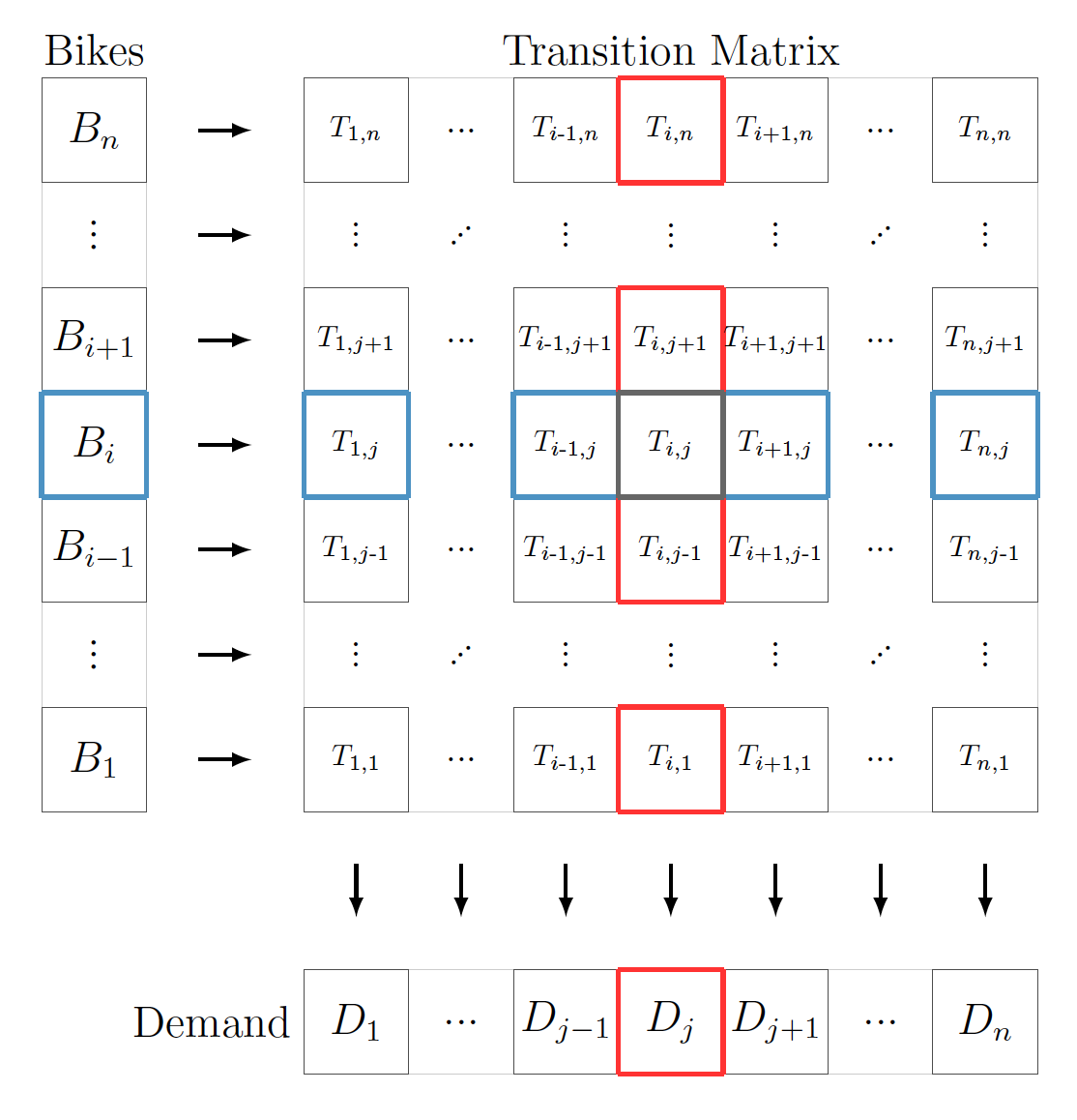
Figure: Bike rebalancing transportation problem: minimize the global transport costs between a set of supply points and a set of demand points. $T_{i,j}\geqslant0$ represents the number of bikes transported from supply point $i$ (with $B_{i}\geqslant0$ bikes available) to demand point $j$ (that requires $D_{j}\geqslant0$ bikes).

References

[1] Brodsky, I., 2018. H3: Uber’s hexagonal hierarchical spatial index. Available from Uber Engineering website: https://eng.uber.com/h3/

[2] Lin, L., He, Z. and Peeta, S., 2018. Predicting station-level hourly demand in a large-scale bike-sharing network: A graph convolutional neural network approach. Transportation Research Part C: Emerging Technologies, 97, pp.258-276

[3] Henaff, M., Bruna, J. and LeCun, Y., 2015. Deep convolutional networks on graph-structured data. arXiv preprint arXiv:1506.05163.